An Analysis of Load Balancing Efficiency

May 31, 2014 § Leave a comment

SUMMARY
In this post, I’m going to examine the properties of different strategies that are commonly used for load-balancing over multiple identical service centres. Common examples of this would be Etherchannel, HTTP load balancers, or applications running on a multicore system.

Unless a load-balancing system is perfect, one of the service centres being balanced will be the most heavily utilized. This service centre is in many ways the most important since, so long it isn’t overloaded, neither are any of the others. We can therefore safely do capacity planning around the properties of the busiest service centre.

The downside of planning on the basis of the busiest service centre is that we are necessarily planning for the other service centres to be under utilized. It is therefore desirable, for the sake of efficiency, that the difference between the utilization of the busiest and the average should be kept to a minimum.

THEORETICAL ANALYSIS
Suppose we have N workloads being balanced over M service centres. A number of load balancing techniques are frequently employed. Typically, a single workload is bound to a single service centre (a), or the individual workloads are broken up into separable units of work, which are then each bound to single service centre, while the original workload is thereby distributed across all the service centres (b). Clearly there is a recursive relationship between (a) and (b). (b) may be broken down into smaller units, which may in turn be broken down again. A theoretical model of (a) then, should be applicable to (b) and so on.

First, we need some estimate of how imperfectly the load is balanced. Suppose the intensity of the work is Normally distributed around the common mean $\lambda$ with standard deviation $\sigma$ . If we examine the combined work in N such workloads, then the intensity will be Normally distributed, such that:
$\sum\limits_{i = 1}^N Normal(\lambda, \sigma^2) = Normal(N \cdot \lambda, N \cdot \sigma^2)$
Equation 1
Meanwhile for each of the M service centres, in case (b), we have:
$\sum\limits_{i = 1}^{\frac{N}{M}} Normal(\lambda, \sigma^2) = Normal(\frac{N}{M} \cdot \lambda, \frac{N}{M} \cdot \sigma^2)$
Equation 2

It can be shown that the expected maximum $E[X]$ from n Normally distributed elements is bounded as follows:
$E[X] \leq \sigma \cdot \sqrt{2 \cdot log(n)}$ ¹
Equation 3

In fact, for $n \geq 4$ the two halves of the inequality are approximately equal:
$E[X] \approxeq \sigma \cdot \sqrt{2 \cdot log(n)}$
Equation 4

So, the difference between the utilization of the maximally busy service centre, and the mean is bounded above and below as follows:
$E[X] \approxeq \sigma\cdot\sqrt{\frac{2 \cdot N \cdot log(M)}{M}}$
Equation 5

Then the maximum utilization is expected to be:
$E[X] \approxeq \frac{N}{M} + \sigma\cdot\sqrt{\frac{2 \cdot N \cdot log(M)}{M}}$
Equation 6

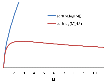
Meanwhile the ratio of excess load of the busiest service centre to the mean is given by:
$E[X] - \frac{N}{M} \approxeq \sigma\cdot\sqrt{\frac{2 \cdot M \cdot log(M)}{N}}$
Equation 7

So, the deviation from the mean is worse for low M before slowly improving due to the reduced mean intensity, meanwhile the deviation as a fraction of the mean increases with M.

Some real world implementations of load balancing distribute load on progressively finer grained quanta. In the case of fibre channel traffic sharing a number of ISLs, an initial course grained approach might allow the routing algorithm to statically assign source/destination pairs to specific links. A better performing approach would be to setup a port-channel and load balance based on source/destination/exchange. But why does load balancing on a smaller quanta improve the efficiency of the load balancing?

It is tempting to suppose that the improvement is due to the reduction in quanta size. If we subdivide each quanta in the previous analysis into $k$ smaller quanta, we see by equation (1) that it is Normally distributed as follow:

$Normal(\frac{\lambda}{k}, \frac{\sigma^2}{k})$
Equation 7

Now, each of the M service centres will be utilized by the combination of $\frac{k \cdot N}{M}$ quanta so, the combined distribution is:

$\sum\limits_{i = 1}^{\frac{k \cdot N}{M}} Normal(\frac{\lambda}{k}, \frac{\sigma^2}{k}) = Normal(\frac{N}{M} \cdot \lambda, \frac{N}{M} \cdot \sigma^2)$
Equation 8

Which is exactly the same distribution as previously. In other words, subdividing the work won’t help, in and of itself.

Why then are smaller divisions of work used in practice to improve balancing efficience? The reason is simple. In order for this strategy to work, there need to exist divisions of work whose standard deviation is less than $\frac{\sigma}{k}$ .

EXAMPLE
In our test environment, I recorded fibre channel traffic on the ingress port of a storage array. The mean exchange size was 20,270 bytes, while the standard deviation was 1586. The same data showed mean frame size of 1861 bytes with a standard deviation of 6.

On average then, each exchange is made up of 11 frames. Using the previous result that for improved load balancing efficiency we need $\sigma_{new} < \frac{\sigma_{old}}{k}$ , we find that $6 < \frac{1586}{11} = 145$ . So, we expect frame level load balancing to be more efficient than exchange level load balancing. In fact it should be around $\frac{145}{6} = 24$ times more efficient.

¹ Performance Modeling for Computer Architects, p.371, C. M. Krishna, 1996

Tagged: Capacity, Load balancing, performance

ascknd