Merging Helpdesks, A Performance Analysis
June 23, 2014 § 2 Comments
I recently encountered a scenario where two helpdesks were to merge. One large, with relatively poor response times, and a smaller one, with relatively good performance. The question was, what would be the impact of merging the call queues on the current customers of the smaller helpdesk? It might seem that the performance of the smaller helpdesk would necessarily be significantly harmed. I’m going to show that that isn’t necessarily the case.
Neil Gunther’s PDQ::Perl1 can be used to do a Mean Value Analysis and predict the impact of combining the queues. That is to say, work out the average performance. I wrote a small Perl script to do this, documented here:
https://ascknd.com/2014/06/23/helpdesk-queue-analyser-pdqperl/
Paradoxically, what we find is that, under certain circumstances, merging the two queues delivers better performance than either helpdesk was capable of delivering on its own:
Example:
Site A has 4 staff working on their queue (e.g. NetApp support), with a call coming in on average every 12.5 minutes. It takes them 30 minutes to deal with each case (excluding time spent in the queue waiting for an operative to become free). At site B they have 6 staff dedicated to a similar queue, who also take 30 minutes to deal with each case, but have an incoming call rate of one call every 5.6 minutes.
Using the previously mentioned script, the behaviour of these helpdesks can be analysed with the following parameters:
perl ./helpdesk_response.pl 4 30 0.08 6 30 .18
What we find is that Site A is 60% utilized and typically only keeps calls waiting in the queue for just over 5 minutes. Site B is 90% utilized and keeps callers waiting in the queue for 37 minutes. When the two queues are combined both sites are 78% utilized and experience waiting times in the queue of <5 minutes. So both sites experience better performance.
How did merging the work of a site with good performance and a site with relatively poor performance lead both sites to improve? Two things are going on:
1. The impact of utilization on performance is non-linear. Moving from 60% utilization to 78% utilization does relatively little harm to site A compared to the benefit experienced by site B.
2. More helpdesk operators are more efficient, from a queueing perspective, than fewer helpdesk operators given the same utilization. That is to say, 6 workers at 60% busy will be more responsive than 4 workers at 60% busy even though in both cases the individual helpdesk operators are performing identically. This is because the more operators there are, the greater the chance that one of them will be free when a call comes in.
Conclusion:
In the general case, one can’t assume that combining the queues of the two helpdesks will necessarily cause the performance of a smaller high performing helpdesk significant harm.
Helpdesk Queue Analyser PDQ::Perl
June 23, 2014 § 1 Comment
Below is a Perl script using the PDQ Perl module to analyser the performance of two helpdesk and predict their behaviour should their queues be merged.
A more complete discussion of the motivations for this and conclusions can be found here:
#/usr/bin/perl
use pdq;
use strict;
use warnings;
my $siteAStaff = $ARGV[0];
my $siteAServiceTime = $ARGV[1];
my $siteARate = $ARGV[2];
my $siteBStaff = $ARGV[3];
my $siteBServiceTime = $ARGV[4];
my $siteBRate = $ARGV[5];
#Handle site A
pdq::Init(“Open Network with M/M/N”);
pdq::SetComment(“Simulation of site A mean performance.”);
pdq::CreateOpen(“work”, $siteARate);
pdq::CreateMultiNode( $siteAStaff, “cores”, $pdq::CEN, $pdq::FCFS);
pdq::SetDemand(“cores”, “work”, $siteAServiceTime);
pdq::SetWUnit(“Calls”);
pdq::SetTUnit(“Mins”);
pdq::Solve($pdq::CANON);
my $responseA = substr(pdq::GetResponse($pdq::TRANS, “work”),0, 8);
my $utilA = substr(pdq::GetUtilization(“cores”, “work”, $pdq::TRANS) * 100,0, 4);
#Handle site B
pdq::Init(“Simulation of site B mean performance.”);
pdq::SetComment(“Simulation of 8 core CPU under transactional load.”);
pdq::CreateOpen(“work”, $siteBRate);
pdq::CreateMultiNode( $siteBStaff, “cores”, $pdq::CEN, $pdq::FCFS);
pdq::SetDemand(“cores”, “work”, $siteBServiceTime);
pdq::SetWUnit(“Calls”);
pdq::SetTUnit(“Mins”);
pdq::Solve($pdq::CANON);
my $responseB = substr(pdq::GetResponse($pdq::TRANS, “work”),0, 8);
my $utilB = substr(pdq::GetUtilization(“cores”, “work”, $pdq::TRANS) * 100,0, 4);
#Handle combined site
pdq::Init(“Open Network with M/M/N”);
pdq::SetComment(“Simulation of comined site mean performance.”);
pdq::CreateOpen(“work”, $siteARate + $siteBRate);
pdq::CreateMultiNode( $siteAStaff + $siteBStaff, “cores”, $pdq::CEN, $pdq::FCFS);
pdq::SetDemand(“cores”, “work”, ($siteAStaff * $siteAServiceTime + $siteBStaff * $siteBServiceTime) / ($siteAStaff + $siteBStaff) );
pdq::SetWUnit(“Calls”);
pdq::SetTUnit(“Mins”);
pdq::Solve($pdq::CANON);
my $responseAB = substr(pdq::GetResponse($pdq::TRANS, “work”),0, 8);
my $utilAB = substr(pdq::GetUtilization(“cores”, “work”, $pdq::TRANS) * 100,0, 4);
printf “Site \t| Response \t | utilization\n”;
printf “A \t| %f \t | % 4d\n”, $responseA, $utilA;
printf “B \t| %f \t | % 4d\n”, $responseB, $utilB;
printf “Combined\t| %f \t | % 4d\n”, $responseAB, $utilAB;
Syntax:
perl ./helpdesk_response.pl <siteA call helpdesk staff#> <siteA service time (mins)> <siteA calls per minute> <siteB call helpdesk staff#> <siteB service time (mins)> <siteB calls per minute>
NB: Service time is used here, not response time, so time spent in the queue doesn’t count. Response time is used in the outputted performance.
Example:
perl ./helpdesk_response.pl 4 30 0.08 6 30 .18
Site | Response | utilization
A | 35.382050 | 60
B | 67.006280 | 90
Combined | 34.990830 | 78
An Analysis of Load Balancing Efficiency
May 31, 2014 § Leave a comment
SUMMARY
In this post, I’m going to examine the properties of different strategies that are commonly used for load-balancing over multiple identical service centres. Common examples of this would be Etherchannel, HTTP load balancers, or applications running on a multicore system.
Unless a load-balancing system is perfect, one of the service centres being balanced will be the most heavily utilized. This service centre is in many ways the most important since, so long it isn’t overloaded, neither are any of the others. We can therefore safely do capacity planning around the properties of the busiest service centre.
The downside of planning on the basis of the busiest service centre is that we are necessarily planning for the other service centres to be under utilized. It is therefore desirable, for the sake of efficiency, that the difference between the utilization of the busiest and the average should be kept to a minimum.
THEORETICAL ANALYSIS
Suppose we have N workloads being balanced over M service centres. A number of load balancing techniques are frequently employed. Typically, a single workload is bound to a single service centre (a), or the individual workloads are broken up into separable units of work, which are then each bound to single service centre, while the original workload is thereby distributed across all the service centres (b). Clearly there is a recursive relationship between (a) and (b). (b) may be broken down into smaller units, which may in turn be broken down again. A theoretical model of (a) then, should be applicable to (b) and so on.
First, we need some estimate of how imperfectly the load is balanced. Suppose the intensity of the work is Normally distributed around the common mean 

Equation 1
Meanwhile for each of the M service centres, in case (b), we have:
Equation 2


It can be shown that the expected maximum ![E[X]](https://s0.wp.com/latex.php?latex=E%5BX%5D&bg=ffffff&fg=222222&s=0&c=20201002)
![E[X] \leq \sigma \cdot \sqrt{2 \cdot log(n)}](https://s0.wp.com/latex.php?latex=E%5BX%5D+%5Cleq+%5Csigma+%5Ccdot+%5Csqrt%7B2+%5Ccdot+log%28n%29%7D&bg=ffffff&fg=222222&s=0&c=20201002)
Equation 3
In fact, for 
Equation 4
![E[X] \approxeq \sigma \cdot \sqrt{2 \cdot log(n)}](https://s0.wp.com/latex.php?latex=E%5BX%5D+%5Capproxeq+%5Csigma+%5Ccdot+%5Csqrt%7B2+%5Ccdot+log%28n%29%7D&bg=ffffff&fg=222222&s=0&c=20201002)
So, the difference between the utilization of the maximally busy service centre, and the mean is bounded above and below as follows:
Equation 5
![E[X] \approxeq \sigma\cdot\sqrt{\frac{2 \cdot N \cdot log(M)}{M}}](https://s0.wp.com/latex.php?latex=E%5BX%5D+%5Capproxeq+%5Csigma%5Ccdot%5Csqrt%7B%5Cfrac%7B2+%5Ccdot+N+%5Ccdot+log%28M%29%7D%7BM%7D%7D&bg=ffffff&fg=222222&s=0&c=20201002)
Then the maximum utilization is expected to be:
Equation 6
![E[X] \approxeq \frac{N}{M} + \sigma\cdot\sqrt{\frac{2 \cdot N \cdot log(M)}{M}}](https://s0.wp.com/latex.php?latex=E%5BX%5D+%5Capproxeq+%5Cfrac%7BN%7D%7BM%7D+%2B+%5Csigma%5Ccdot%5Csqrt%7B%5Cfrac%7B2+%5Ccdot+N+%5Ccdot+log%28M%29%7D%7BM%7D%7D&bg=ffffff&fg=222222&s=0&c=20201002)
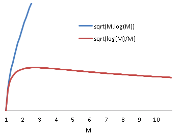
Meanwhile the ratio of excess load of the busiest service centre to the mean is given by:
Equation 7
![E[X] - \frac{N}{M} \approxeq \sigma\cdot\sqrt{\frac{2 \cdot M \cdot log(M)}{N}}](https://s0.wp.com/latex.php?latex=E%5BX%5D+-+%5Cfrac%7BN%7D%7BM%7D+%5Capproxeq+%5Csigma%5Ccdot%5Csqrt%7B%5Cfrac%7B2+%5Ccdot+M+%5Ccdot+log%28M%29%7D%7BN%7D%7D&bg=ffffff&fg=222222&s=0&c=20201002)
So, the deviation from the mean is worse for low M before slowly improving due to the reduced mean intensity, meanwhile the deviation as a fraction of the mean increases with M.
Some real world implementations of load balancing distribute load on progressively finer grained quanta. In the case of fibre channel traffic sharing a number of ISLs, an initial course grained approach might allow the routing algorithm to statically assign source/destination pairs to specific links. A better performing approach would be to setup a port-channel and load balance based on source/destination/exchange. But why does load balancing on a smaller quanta improve the efficiency of the load balancing?
It is tempting to suppose that the improvement is due to the reduction in quanta size. If we subdivide each quanta in the previous analysis into 
Equation 7

Now, each of the M service centres will be utilized by the combination of 
Equation 8

Which is exactly the same distribution as previously. In other words, subdividing the work won’t help, in and of itself.
Why then are smaller divisions of work used in practice to improve balancing efficience? The reason is simple. In order for this strategy to work, there need to exist divisions of work whose standard deviation is less than 
EXAMPLE
In our test environment, I recorded fibre channel traffic on the ingress port of a storage array. The mean exchange size was 20,270 bytes, while the standard deviation was 1586. The same data showed mean frame size of 1861 bytes with a standard deviation of 6.
On average then, each exchange is made up of 11 frames. Using the previous result that for improved load balancing efficiency we need 


1 Performance Modeling for Computer Architects, p.371, C. M. Krishna, 1996
Perl PDQ: 8 core response time under load
May 15, 2014 § 1 Comment
The following Perl PDQ1; script was used to generate the response time data for the 8 core example in my https://ascknd.com/2014/05/02/nfs-vs-fibre-cpu-vmware/ post:
#/usr/bin/perl
use pdq;
$cores = $ARGV[0];
$servTime = $ARGV[1];
$max_rate = (1 / $servTime) * $cores;
print “response(secs)\t | util_%\n”;
for ($rate = 0; $rate < $max_rate ; $rate += $max_rate / 5) {
$arrivRate = $rate;
pdq::Init(“Open Network with M/M/N”);
pdq::SetComment(“Simulation of N CPU cores under transactional load.”);
pdq::CreateOpen(“work”, $arrivRate);
pdq::CreateMultiNode( $cores, “cores”, $pdq::CEN, $pdq::FCFS);
pdq::SetDemand(“cores”, “work”, $servTime);
pdq::SetWUnit(“IOS”);
pdq::SetTUnit(“Secs”);
pdq::Solve($pdq::CANON);
$response = substr(pdq::GetResponse($pdq::TRANS, “work”),0, 8);
$util = substr(pdq::GetUtilization(“cores”, “work”, $pdq::TRANS) * 100,0, 4);
printf “$response \t | % 4d\n”, $util;
}
perl ./mm8_response.pl 8 0.000127
response(secs) | util_%
0.000127 | 0
0.000127 | 20
0.000127 | 40
0.000132 | 60
0.000163 | 80
NFS vs Fibre Channel: Comparing CPU Utilization in VMWare
May 2, 2014 § 3 Comments
SUMMARY
Some years ago we were faced with the choice of which storage network protocol to use in our virtualized environment. Central to the discussion was a white paper, co-authored by Netapp and VMWare, comparing throughput and CPU utilization for NFS, FC and iSCSI. Broadly speaking the paper concluded that the differences in throughput were trivial, and for CPU utilization were under most circumstances small. At the time I wasn’t satisfied with the document, or indeed the conclusions that were able to drawn from it.
In this post, I will outline some work I performed recently using Queuing Theory1 and Design of Experiments2 to draw more specific conclusions from a broadly similar set of experiments to those undertaken by NetApp. I show that, if we restrict our analysis to storage efficiency in the hypervisor, in fact the choice of protocol is the dominant influence on CPU load, after IOPS (as can clearly be seen below in figure 4), and that under some circumstances, where latency of the order of 100μs is significant, or the total volume of IO is large, the choice of protocol can be an important determinant of performance, and potentially cost.
LIMITATIONS OF THE NETAPP PAPER
The white paper in question is NetApp document TR-36973. The equipment is more than a little out of date now, ESX 3.5, GigE, NetApp 2000 and 3000 series boxes and 2Gb FC-AL fibre. They ran 4K and 8K random and sequential workloads at various read/write ratios and at a range of thread counts. Tests were run to compare workloads over NFS, FC and iSCSI. For the purpose of this analysis, I ignore iSCSI and concentrate on NFS and FC.
In making use of this paper some issues become apparent:
1. All experimental results are scaled with respect to FC. This makes it hard to get a sense of what the result means in real terms, or to compare results between experiments.
2. The IOPS aren’t fixed between, or within, experiments. If response times increase, the IOPS, and hence the throughput, will tend to drop. This is observed in the results with NFS producing somewhat less throughput than FC under increased load.
If the IOPS are suppressed for NFS, then we might expect this also to keep the CPU utilization down, since there are fewer IOs for the CPU to process per unit of time. Despite this, the CPU is working harder for NFS.
3. By throttling based on the thread count, they are implicitly assuming closed queuing. This is not necessarily applicable to modeling transactional workloads.
4. Due to caching and interaction with the filesystem, it isn’t clear what IO is being processed by the VMWare IO subsystem. This will tend to minimize differences in the performance of the underlying infrastructure, since it is only being used a proportion of the time.
To progress with the analysis, fresh data is needed.
STEP 1: Test Configuration
I set up a small test configuration to run a similar set of experiments to those in the paper, though this time just comparing NFS and FC. There are some significant differences between the setup NetApp used and the one I built. Partly that is because technology has moved on since 2008, but most of the changes are because I have simplified the setup as far as possible.
The physical setup was as follows:

Figure 1
I ran a single minimally configured Debian guest running the 3.2.0-4-686-pae kernel inside an ESXi 5.5 (1331820) hypervisor. I configured a disk from an NFS datastore, and one from an FC datastore. The guest was assigned 8 vCPU and 1GB of memory.
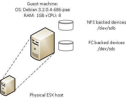
Figure 2
STEP 2: Workload Generation
In their test, NetApp used Iometer4 which throttles the workload based on thread count. Most freely available tools operate along the same lines as Iometer. To achieve the required level of control, I modified NetApp’s sio_ntap5 to hold a specified level of IOPS. A more detailed description of this work can be found here:
https://ascknd.com/2014/05/28/616/
I ran sio_ntap with the directio option set, bypassing cache and directed to a raw device. By doing this, different factors that directly influency the intensity of the workload can be compared and their effect quantified.
STEP 3: Experimental Design
NetApp consider a number of factors in their analysis – read%, random%, block size, protocol and thread count. I’m going to substitute IOPS for thread count. The response we are interested in is the CPU used by the ESX kernel (
In order to formulate a model of this system, it is necessary to make some assumptions:
1. An IO of any given type will take a fixed amount of CPU resources regardless of load.
1.1 We therefore expect to see all effects to involve a linear interaction with IOPS. This can readily be validated by plotting a graph showing the percentage of a CPU core used by the ESX kernel, as discussed above, for various workloads and IOPS:

Figure 3
It can readily be seen that NFS and FC diverge with plausibly linear behavior.
1.2 For any given read percent, or random percent, an IO is either read or write, random or sequential. We therefore expect their effect to be linear.
2. Since we are only interested in block sizes of 4 or 8, we will only consider linear effects of block size. No claims are made about applicability of the model to larger block sizes
3. Some background load will exist. This is assumed to be the load for zero IOPS. This will be deducted from all subsequent calculations for CPU load. Taking this into account, the previous graph can be amended so that the average CPU utilization at zero IOPS is zero:

Figure 4
All effects are therefore expected to be linear, to involve interactions with IOPS and go through the origin.
The following design will be used:
| read% | rand% | blk_sz | protocol | iops |
| 0 | 0 | 4 | fc | 1000 |
| 100 | 100 | 8 | nfs | 4000 |
Table 1
This gives a full factorial experimental design with 32 experiments. Repeating every experiment 20 times, 640 runs are needed.
| run | read% | rand% | blk_sz | protocol | iops |
| 1 | 0 | 100 | 4 | fc | 4000 |
| 2 | 0 | 0 | 8 | fc | 1000 |
| <snip> | |||||
| 639 | 0 | 0 | 4 | fc | 4000 |
| 640 | 0 | 0 | 8 | nfs | 1000 |
Table 2
A more detailed discussion on how to create the design in R is shown here:
We now need to run the modified sio_ntap tool with the above parameters 640 times and analyze the results.
STEP 4: Analysis of Results
R6 is used with the DoE7 package to analyze the results. This solves the experimental results as a system of simultaneous equation. A detailed explanation of this is presented here:
The analysis shows that we can approximate the CPU utilization, by the following equation for large IOPS:
Equation 1

Which implies that NFS is approximately 1.96 times as expensive in terms of CPU utilization as Fibre Channel (see linked article).
STEP 5: Real World Context
Whether this difference in the cost of NFS and FC IO is important, or not, depends on the extent to which it has a significant impact on macro level system characteristics that relate to the financial cost, and feasibility, of delivering on design requirements.
Solving equation 1 for a single IOP, we see that one NFS IO uses 
| response(secs) | util_% |
| 0.000081 | 0 |
| 0.000081 | 20 |
| 0.000081 | 40 |
| 0.000085 | 60 |
| 0.000104 | 80 |
Table 3
A typical midrange disk subsystem can turn around an IO in about 500μs. Some higher end subsystems can respond in 150μs, or less. So this is an effect that is of the same order of magnitude as other metrics that clearly can determine system performance.
These individual IOs add up of course. In this example, one CPU core can handle ~12K NFS IOPS, or 24K FC IOPS. This potentially has architectural and cost implications if a significant intensity of IO is being serviced. A 70K IOP requirement would require a 6 cores for NFS, but only 3 for FC, purely processing the IO in the hypervisor.
CONCLUSIONS
While NFS clearly induces more load on the ESX server than FC, to some degree these costs need to be seen in context. The reason the NetApp paper found a relatively small difference between the protocols is that there are many other factors contribute to the overall CPU load associated with doing IO. Often the cost within the hypervisor will be relatively insignificant:
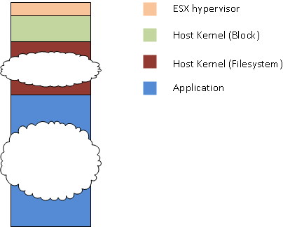
Figure 5
Whether the hypervisor is important depends on the interaction between the workload and each of these other elements. Analysing these interactions is a larger problem and not trivial to address in the general case.
1The Art of Computer Systems Performance Analysis, p.507 R. Jain, John Wiley & Sons Inc, 1991
2The Art of Computer Systems Performance Analysis, p.293 R. Jain, John Wiley & Sons Inc, 1991
3 Performance Report: Multiprotocol Performance Test of VMware® ESX 3.5 on NetApp Storage Systems, https://communities.vmware.com/servlet/JiveServlet/download/1085778-15260/NetApp_PerformanceTest_tr-3697.pdf, Jack McLeod, NetApp, June 2008
4 http://www.iometer.org/
5 https://communities.netapp.com/blogs/zurich/2011/01/24/sio–performance-load-testing-simplified
6 http://cran.r-project.org/
7 http://prof.beuth-hochschule.de/groemping/software/design-of-experiments/project-industrial-doe-in-r/
8 https://ascknd.com/2014/05/15/442/
Document Changes:
27/05/2014 – Updated experimental design with 20 replications instead of 5 and simplified the setup of the block devices. All equations and graphs modified to agree with new data. Some additional minor cosmetic changes and corrections.
