ascknd

As load increases on a service center, in the case of our earlier example – a fibre channel port, queues of requests form. These queues are held in the buffers of the port. In my first post, I assumed that the buffers were infinitely deep. That is clearly not the case for any real world implementation. Historically in fibre channel networks relatively few buffers were used when compared to Ethernet networks. Cisco has tended to have more buffers than Brocade. A typical value for Cisco is shown here: 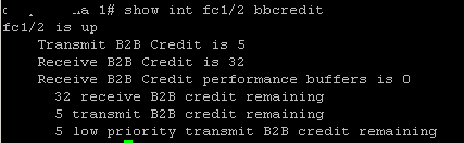We see 32 bbcredits. While for Brocade: there are only 8. Of course higher values are common, and often essential, for ISLs over distance, but these are fairly typical values. So, how do these numbers impact the performance of the 8Gb/s port in our model. We can use Little’s law to work out the queue length.

Where L is the mean requests in the queue, is the arrival rate, and W is the total time the request is in the queue. It can immediately be seen that , so:

Now, the arrival rate must be:

So, we now have:

and substituting back in the M/M/1 queuing formula from my previous post, we have:

Now, simplifying, we get a formula for the queue length wrt utilization and service time.

We can now graph the relationship between queue length and utilization for a service time of 2.5 microseconds:

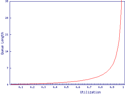
We find that the port with 8 buffers runs out of bbcredits just before 90% utilization, while the port with 32 buffers makes it to 97%. In and of itself a 7% difference in how heavily the port can be loaded may not be particularly important. It is after all only 573Mb/s, however, it may have wider implications for the fibre channel network due to the way buffer credits work.

Tagged: fibre channel, performance, Queuing Theory