Helpdesk Queue Analyser PDQ::Perl
June 23, 2014 § 1 Comment
Below is a Perl script using the PDQ Perl module to analyser the performance of two helpdesk and predict their behaviour should their queues be merged.
A more complete discussion of the motivations for this and conclusions can be found here:
#/usr/bin/perl
use pdq;
use strict;
use warnings;
my $siteAStaff = $ARGV[0];
my $siteAServiceTime = $ARGV[1];
my $siteARate = $ARGV[2];
my $siteBStaff = $ARGV[3];
my $siteBServiceTime = $ARGV[4];
my $siteBRate = $ARGV[5];
#Handle site A
pdq::Init(“Open Network with M/M/N”);
pdq::SetComment(“Simulation of site A mean performance.”);
pdq::CreateOpen(“work”, $siteARate);
pdq::CreateMultiNode( $siteAStaff, “cores”, $pdq::CEN, $pdq::FCFS);
pdq::SetDemand(“cores”, “work”, $siteAServiceTime);
pdq::SetWUnit(“Calls”);
pdq::SetTUnit(“Mins”);
pdq::Solve($pdq::CANON);
my $responseA = substr(pdq::GetResponse($pdq::TRANS, “work”),0, 8);
my $utilA = substr(pdq::GetUtilization(“cores”, “work”, $pdq::TRANS) * 100,0, 4);
#Handle site B
pdq::Init(“Simulation of site B mean performance.”);
pdq::SetComment(“Simulation of 8 core CPU under transactional load.”);
pdq::CreateOpen(“work”, $siteBRate);
pdq::CreateMultiNode( $siteBStaff, “cores”, $pdq::CEN, $pdq::FCFS);
pdq::SetDemand(“cores”, “work”, $siteBServiceTime);
pdq::SetWUnit(“Calls”);
pdq::SetTUnit(“Mins”);
pdq::Solve($pdq::CANON);
my $responseB = substr(pdq::GetResponse($pdq::TRANS, “work”),0, 8);
my $utilB = substr(pdq::GetUtilization(“cores”, “work”, $pdq::TRANS) * 100,0, 4);
#Handle combined site
pdq::Init(“Open Network with M/M/N”);
pdq::SetComment(“Simulation of comined site mean performance.”);
pdq::CreateOpen(“work”, $siteARate + $siteBRate);
pdq::CreateMultiNode( $siteAStaff + $siteBStaff, “cores”, $pdq::CEN, $pdq::FCFS);
pdq::SetDemand(“cores”, “work”, ($siteAStaff * $siteAServiceTime + $siteBStaff * $siteBServiceTime) / ($siteAStaff + $siteBStaff) );
pdq::SetWUnit(“Calls”);
pdq::SetTUnit(“Mins”);
pdq::Solve($pdq::CANON);
my $responseAB = substr(pdq::GetResponse($pdq::TRANS, “work”),0, 8);
my $utilAB = substr(pdq::GetUtilization(“cores”, “work”, $pdq::TRANS) * 100,0, 4);
printf “Site \t| Response \t | utilization\n”;
printf “A \t| %f \t | % 4d\n”, $responseA, $utilA;
printf “B \t| %f \t | % 4d\n”, $responseB, $utilB;
printf “Combined\t| %f \t | % 4d\n”, $responseAB, $utilAB;
Syntax:
perl ./helpdesk_response.pl <siteA call helpdesk staff#> <siteA service time (mins)> <siteA calls per minute> <siteB call helpdesk staff#> <siteB service time (mins)> <siteB calls per minute>
NB: Service time is used here, not response time, so time spent in the queue doesn’t count. Response time is used in the outputted performance.
Example:
perl ./helpdesk_response.pl 4 30 0.08 6 30 .18
Site | Response | utilization
A | 35.382050 | 60
B | 67.006280 | 90
Combined | 34.990830 | 78
Net Present Value
June 13, 2014 § Leave a comment
When working in IT, one frequently encounters situations where a purchasing decision needs to be made whose costs and benefits occur over an extended period of time. In my organization, we typically look at such things over three years. Under such circumstances the relative value of money now, as opposed to money in the future, becomes important.
If you have a pound today, you could invest it (in the market, say) or put it to work doing something that produces some ‘return on investment’. After a year you can expect your pound to be worth one pound + the return on investment. In other words, a pound now is better than a pound deferred until tomorrow.
Net Present Value attempts to adjust for this effect. It is calculated as follows:
where 


Say we know we must pay £100,000 per year in ongoing support costs on a storage array and the return on the money that we would otherwise expect to get is 10%.


In this analysis then, a prospective replacement disk subsystem would need to cost less than £273,554 to save money over the three years considered.
This is a simplification of course. The old and new subsystems probably have different costs in terms of heat and power to name just two other things that could be factored in.
An Analysis of Load Balancing Efficiency
May 31, 2014 § Leave a comment
SUMMARY
In this post, I’m going to examine the properties of different strategies that are commonly used for load-balancing over multiple identical service centres. Common examples of this would be Etherchannel, HTTP load balancers, or applications running on a multicore system.
Unless a load-balancing system is perfect, one of the service centres being balanced will be the most heavily utilized. This service centre is in many ways the most important since, so long it isn’t overloaded, neither are any of the others. We can therefore safely do capacity planning around the properties of the busiest service centre.
The downside of planning on the basis of the busiest service centre is that we are necessarily planning for the other service centres to be under utilized. It is therefore desirable, for the sake of efficiency, that the difference between the utilization of the busiest and the average should be kept to a minimum.
THEORETICAL ANALYSIS
Suppose we have N workloads being balanced over M service centres. A number of load balancing techniques are frequently employed. Typically, a single workload is bound to a single service centre (a), or the individual workloads are broken up into separable units of work, which are then each bound to single service centre, while the original workload is thereby distributed across all the service centres (b). Clearly there is a recursive relationship between (a) and (b). (b) may be broken down into smaller units, which may in turn be broken down again. A theoretical model of (a) then, should be applicable to (b) and so on.
First, we need some estimate of how imperfectly the load is balanced. Suppose the intensity of the work is Normally distributed around the common mean 

Equation 1
Meanwhile for each of the M service centres, in case (b), we have:
Equation 2


It can be shown that the expected maximum ![E[X]](https://s0.wp.com/latex.php?latex=E%5BX%5D&bg=ffffff&fg=222222&s=0&c=20201002)
![E[X] \leq \sigma \cdot \sqrt{2 \cdot log(n)}](https://s0.wp.com/latex.php?latex=E%5BX%5D+%5Cleq+%5Csigma+%5Ccdot+%5Csqrt%7B2+%5Ccdot+log%28n%29%7D&bg=ffffff&fg=222222&s=0&c=20201002)
Equation 3
In fact, for 
Equation 4
![E[X] \approxeq \sigma \cdot \sqrt{2 \cdot log(n)}](https://s0.wp.com/latex.php?latex=E%5BX%5D+%5Capproxeq+%5Csigma+%5Ccdot+%5Csqrt%7B2+%5Ccdot+log%28n%29%7D&bg=ffffff&fg=222222&s=0&c=20201002)
So, the difference between the utilization of the maximally busy service centre, and the mean is bounded above and below as follows:
Equation 5
![E[X] \approxeq \sigma\cdot\sqrt{\frac{2 \cdot N \cdot log(M)}{M}}](https://s0.wp.com/latex.php?latex=E%5BX%5D+%5Capproxeq+%5Csigma%5Ccdot%5Csqrt%7B%5Cfrac%7B2+%5Ccdot+N+%5Ccdot+log%28M%29%7D%7BM%7D%7D&bg=ffffff&fg=222222&s=0&c=20201002)
Then the maximum utilization is expected to be:
Equation 6
![E[X] \approxeq \frac{N}{M} + \sigma\cdot\sqrt{\frac{2 \cdot N \cdot log(M)}{M}}](https://s0.wp.com/latex.php?latex=E%5BX%5D+%5Capproxeq+%5Cfrac%7BN%7D%7BM%7D+%2B+%5Csigma%5Ccdot%5Csqrt%7B%5Cfrac%7B2+%5Ccdot+N+%5Ccdot+log%28M%29%7D%7BM%7D%7D&bg=ffffff&fg=222222&s=0&c=20201002)
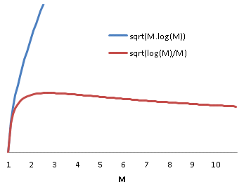
Meanwhile the ratio of excess load of the busiest service centre to the mean is given by:
Equation 7
![E[X] - \frac{N}{M} \approxeq \sigma\cdot\sqrt{\frac{2 \cdot M \cdot log(M)}{N}}](https://s0.wp.com/latex.php?latex=E%5BX%5D+-+%5Cfrac%7BN%7D%7BM%7D+%5Capproxeq+%5Csigma%5Ccdot%5Csqrt%7B%5Cfrac%7B2+%5Ccdot+M+%5Ccdot+log%28M%29%7D%7BN%7D%7D&bg=ffffff&fg=222222&s=0&c=20201002)
So, the deviation from the mean is worse for low M before slowly improving due to the reduced mean intensity, meanwhile the deviation as a fraction of the mean increases with M.
Some real world implementations of load balancing distribute load on progressively finer grained quanta. In the case of fibre channel traffic sharing a number of ISLs, an initial course grained approach might allow the routing algorithm to statically assign source/destination pairs to specific links. A better performing approach would be to setup a port-channel and load balance based on source/destination/exchange. But why does load balancing on a smaller quanta improve the efficiency of the load balancing?
It is tempting to suppose that the improvement is due to the reduction in quanta size. If we subdivide each quanta in the previous analysis into 
Equation 7

Now, each of the M service centres will be utilized by the combination of 
Equation 8

Which is exactly the same distribution as previously. In other words, subdividing the work won’t help, in and of itself.
Why then are smaller divisions of work used in practice to improve balancing efficience? The reason is simple. In order for this strategy to work, there need to exist divisions of work whose standard deviation is less than 
EXAMPLE
In our test environment, I recorded fibre channel traffic on the ingress port of a storage array. The mean exchange size was 20,270 bytes, while the standard deviation was 1586. The same data showed mean frame size of 1861 bytes with a standard deviation of 6.
On average then, each exchange is made up of 11 frames. Using the previous result that for improved load balancing efficiency we need 


1 Performance Modeling for Computer Architects, p.371, C. M. Krishna, 1996
Modified IO Load Generator (sio_ntap.c)
May 28, 2014 § 1 Comment
Below is the text of a diff output between the NetApp sio_ntap.c file, downloadable from here:
https://communities.netapp.com/blogs/zurich/2011/01/24/sio–performance-load-testing-simplified
and my updated version. To merge them, “patch ./sio_ntap ./sio_ntap.c.diff” should be sufficient.
The ammended version attempts to produce a specified number of IOPS by throttling a sleep. Once the required rate has been successfully held, the sleep time is fixed for the duration of the measured run.
An extension to this would be to alter the distribution of the sleep time to approximate a Poisson process. This should give more realistic performance figures under load.
44,45c44
< #include <unistd.h> // need for usleep
< #include <time.h> // need for nanosecond timer
—
>
115,116c114
< #define IOPS_POS 7
< #define DEVICES_POS 8
—
> #define DEVICES_POS 7
135,137d132
< pthread_mutex_t mutx = PTHREAD_MUTEX_INITIALIZER;
< pthread_cond_t condx = PTHREAD_COND_INITIALIZER;
< typedef enum { false, true } bool;
153c148
< struct timeb begin_time, end_time, cur_time, tmp_time;
—
> struct timeb begin_time, end_time;
169,187d163
< struct timespec timer_start() {
< struct timespec start_time_ns;
< clock_gettime(CLOCK_REALTIME, &start_time_ns);
< return start_time_ns;
< }
<
< long timer_end(struct timespec start_time_ns) {
< struct timespec end_time_ns;
< clock_gettime(CLOCK_REALTIME, &end_time_ns);
< long diffInNs = end_time_ns.tv_nsec – start_time_ns.tv_nsec;
< if ( start_time_ns.tv_nsec > end_time_ns.tv_nsec ) {
< diffInNs += 1000000000; //adjust for having times from different seconds.
< }
< return diffInNs;
< }
<
<
<
<
241d216
< int iops_target = atoi (argv[IOPS_POS]);
266,267d240
<
< int sleep_us = 1000 * 1000 / iops_target;
269c242
< while (!io_completes[i]) {
—
> while (!io_completes[i])
271d243
< }
279,340c251
< ftime (&cur_time);
< int iops_counter = 0;
<
< long time_elapsed_ns = 0;
<
< struct timespec run_start_time = timer_start();
< bool in_warmup = true;
< bool in_speedtest = false;
< int iops_scale_pct = 100;
< int hold_count = 0;
<
< printf(“Beginning warmup phase. Attempting to hold requested mean IO rate.\n”);
< while(cur_time.time – begin_time.time < run_time ) {
<
< //Need to spend the first second working out what the scale factor needs to be….
< if (in_warmup == true && timer_end(run_start_time) > 900000000L ) {
< //Done warmup
< in_warmup = false;
< in_speedtest = true;
< iops_counter = 0;
< run_start_time = timer_start();
< }
< if (in_speedtest == true && timer_end( run_start_time) > 900000000L ) {
< int tmp_iops_scale_pct = 90 * iops_target / iops_counter;
< if (tmp_iops_scale_pct <= 100) {
< //No more scaling needed.
< ++hold_count;
< if (hold_count == 10) {
< in_speedtest = false;
< for (i = 0; i < num_threads; i++) io_completes[i] = 0;
< in_speedtest = false;
< in_warmup = false;
< }
< else {
< in_speedtest = false;
< in_warmup = true;
< }
< } else {
< in_warmup = true;
< in_speedtest = false;
< }
<
< //Only change scale factor if > 100.
< //if (tmp_iops_scale_pct > 100)
< iops_scale_pct = iops_scale_pct * tmp_iops_scale_pct / 100;
< printf(“.”);
< run_start_time = timer_start();
< iops_counter = 0;
<
< //reset timers so this doesn’t count to run length, or to iops.
< ftime (&begin_time);
< }
<
< struct timespec loop_start_time = timer_start();
< usleep (sleep_us * 100 / iops_scale_pct);
< pthread_cond_signal(&condx);
< ++iops_counter;
< ftime (&cur_time);
< time_elapsed_ns = timer_end( loop_start_time );
< }
< printf(“\n”);
<
—
> sleep (run_time);
484a396
>
519,523d430
<
< //Setup threading to wait for io.
< pthread_mutex_lock (&mutx);
< pthread_cond_wait(&condx, &mutx);
< pthread_mutex_unlock(&mutx);
Note: This patch has only been tested on Linux.
Analysing Experimental Results With R
May 27, 2014 § 2 Comments
In this post, I will briefly show an analysis of the results of the experimental design I created earlier:
Creating an Experimental Design in R
The design concerns the interactions between storage protocol, iops, read%, rand% and block size for IO in VMWare. The effect under analysis is the CPU utilization of the ESX kernel. The motivation for this is discussed here:
NFS vs Fibre Channel: Comparing CPU Utilization in VMWare
I load the previous experimental design, having added a response column:
load( “V:/Doe/Design.1.rda” )
Design.1.withresp <- add.response(Design.1,
“V:/Doe/Design.1.with_response.csv”, replace=FALSE)
Now, apply linear regression and summarize the results:
LinearModel.1 <- lm(cpu ~ (read + rand + blk_sz + protocol + iops)^2,
data=Design.1.withresp)
summary(LinearModel.1)
This produces the following table:
Coefficients:
Estimate Std. Error t value Pr(>|t|)
(Intercept) 3.256812 0.018130 179.632 < 2e-16 ***
read1 -0.074656 0.018130 -4.118 4.34e-05 ***
rand1 -0.001125 0.018130 -0.062 0.95054
blk_sz1 0.040906 0.018130 2.256 0.02440 *
protocol1 0.608219 0.018130 33.547 < 2e-16 ***
iops1 1.032375 0.018130 56.942 < 2e-16 ***
read1:rand1 -0.016969 0.018130 -0.936 0.34967
read1:blk_sz1 -0.018875 0.018130 -1.041 0.29825
read1:protocol1 -0.006219 0.018130 -0.343 0.73171
read1:iops1 -0.110219 0.018130 -6.079 2.10e-09 ***
rand1:blk_sz1 -0.017750 0.018130 -0.979 0.32795
rand1:protocol1 -0.002937 0.018130 -0.162 0.87134
rand1:iops1 0.005656 0.018130 0.312 0.75516
blk_sz1:protocol1 0.062063 0.018130 3.423 0.00066 ***
blk_sz1:iops1 0.026219 0.018130 1.446 0.14865
protocol1:iops1 0.369719 0.018130 20.392 < 2e-16 ***
—
Signif. codes: 0 ‘***’ 0.001 ‘**’ 0.01 ‘*’ 0.05 ‘.’ 0.1 ‘ ‘ 1
Residual standard error: 0.4587 on 624 degrees of freedom
Multiple R-squared: 0.8862, Adjusted R-squared: 0.8835
F-statistic: 324 on 15 and 624 DF, p-value: < 2.2e-16
The most immediately useful column is the estimate of the coefficient. If we assume that the CPU utilization is given by an equation of the form:
In this case, we see that 


Meanwhile, each of the factors is normalized so that the low value corresponds to -1, and the high value to +1. So, we have:
Where protocol is -1 in the case of fibre channel and +1 in the case of NFS.

As load increases, we expect the CPU utilization to be dominated by effects involving relationships with IOPS. That is to say, if 

So, we can simplify things be ignoring all effects not involving IOPS, giving the following formula for CPU utilization:

The terms involving interactions with rand and block size clearly have relatively little impact, so I discard them with minimal loss in precision.


In the original experiment, the CPU utilization was calculated for 8 cores. Normalizing for a single core, we have:

It is now also possible to approximate the CPU cost of NFS over fibre channel:

With the minimum difference for write IO, and the maximum for read.
So, in this experiment, NFS is found to be of the order of twice as expensive as fibre channel.
