fibre channel | ascknd

Analysing Experimental Results With R

May 27, 2014 § 2 Comments

In this post, I will briefly show an analysis of the results of the experimental design I created earlier:
Creating an Experimental Design in R

The design concerns the interactions between storage protocol, iops, read%, rand% and block size for IO in VMWare. The effect under analysis is the CPU utilization of the ESX kernel. The motivation for this is discussed here:
NFS vs Fibre Channel: Comparing CPU Utilization in VMWare

I load the previous experimental design, having added a response column:
load( “V:/Doe/Design.1.rda” )
Design.1.withresp <- add.response(Design.1,
“V:/Doe/Design.1.with_response.csv”, replace=FALSE)

Now, apply linear regression and summarize the results:
LinearModel.1 <- lm(cpu ~ (read + rand + blk_sz + protocol + iops)^2,
data=Design.1.withresp)
summary(LinearModel.1)

This produces the following table:

Coefficients:
Estimate Std. Error t value Pr(>|t|)
(Intercept)        3.256812   0.018130 179.632 < 2e-16 ***
read1             -0.074656   0.018130 -4.118 4.34e-05 ***
rand1             -0.001125   0.018130 -0.062 0.95054
blk_sz1            0.040906   0.018130   2.256 0.02440 *
protocol1          0.608219   0.018130 33.547 < 2e-16 ***
iops1              1.032375   0.018130 56.942 < 2e-16 ***
read1:rand1       -0.016969   0.018130 -0.936 0.34967
read1:blk_sz1     -0.018875   0.018130 -1.041 0.29825
read1:protocol1   -0.006219   0.018130 -0.343 0.73171
read1:iops1       -0.110219   0.018130 -6.079 2.10e-09 ***
rand1:blk_sz1     -0.017750   0.018130 -0.979 0.32795
rand1:protocol1   -0.002937   0.018130 -0.162 0.87134
rand1:iops1        0.005656   0.018130   0.312 0.75516
blk_sz1:protocol1 0.062063   0.018130   3.423 0.00066 ***
blk_sz1:iops1      0.026219   0.018130   1.446 0.14865
protocol1:iops1    0.369719   0.018130 20.392 < 2e-16 ***
—
Signif. codes: 0 ‘***’ 0.001 ‘**’ 0.01 ‘*’ 0.05 ‘.’ 0.1 ‘ ‘ 1

Residual standard error: 0.4587 on 624 degrees of freedom
Multiple R-squared: 0.8862, Adjusted R-squared: 0.8835
F-statistic: 324 on 15 and 624 DF, p-value: < 2.2e-16

The most immediately useful column is the estimate of the coefficient. If we assume that the CPU utilization is given by an equation of the form:

$ESX_{CPU} = Intercept + \alpha_1 \cdot read1 + \alpha_2 \cdot rand1 + \textellipsis + \alpha_n \cdot protocol1 \cdot iops1$
In this case, we see that $Intercept = 3.256812$ , $\alpha_1 = -0.074656$ and so on for all the coefficients.

Meanwhile, each of the factors is normalized so that the low value corresponds to -1, and the high value to +1. So, we have:
$ESX_{CPU} = 3.256812 - 0.074656 \cdot \frac{read - 50}{50} - 0.001125 \cdot \frac{rand - 50}{50} + \textellipsis + 0.369719 \cdot protocol \cdot \frac{iops - 2500}{1500}$
Where protocol is -1 in the case of fibre channel and +1 in the case of NFS.

As load increases, we expect the CPU utilization to be dominated by effects involving relationships with IOPS. That is to say, if $ESX_{{CPU}_{APPROX}} is ESX_{CPU}$ without the terms not involving IOPS:

$\lim \limits_{IOPS \to \infty} \frac{ESX_{{CPU}_{APPROX}}- ESX_{CPU}}{ESX_{CPU}} = 0$

So, we can simplify things be ignoring all effects not involving IOPS, giving the following formula for CPU utilization:
$ESX_{{CPU}_{APPROX}} = 1.032375 \cdot \frac{iops}{1500} - 0.110219 \cdot \frac{read - 50}{50} \cdot \frac{iops}{1500} + 0.005656 \cdot \frac{rand - 50}{50} \cdot \frac{iops}{1500} + 0.026219 \cdot \frac{blksz - 6}{2} \cdot \frac{iops}{1500} + 0.369719 \cdot protocol \cdot \frac{iops}{1500}$

The terms involving interactions with rand and block size clearly have relatively little impact, so I discard them with minimal loss in precision.

$ESX_{{CPU}_{APPROX}} \approx 7.6173 \cdot 10^{-4} \cdot iops - 1.4696 \cdot 10 ^ {-6} \cdot read \cdot iops + 2.4648 \cdot 10^{-4} \cdot protocol \cdot iops$

$ESX_{{CPU}_{APPROX}} \approx 7.6173 \cdot 10^{-4} \cdot iops \cdot (1 - 1.9293 \cdot 10 ^ {-3} \cdot read + 0.3236 \cdot protocol)$

In the original experiment, the CPU utilization was calculated for 8 cores. Normalizing for a single core, we have:

$ESX_{{CPU^1}_{APPROX}} \approx 60.9384 \cdot 10^{-4} \cdot iops \cdot (1 - 1.9293 \cdot 10 ^ {-3} \cdot read + 0.3236 \cdot protocol)$

It is now also possible to approximate the CPU cost of NFS over fibre channel:

$1.96 < \frac{NFS cost}{FC cost} < 2.34$

With the minimum difference for write IO, and the maximum for read.

So, in this experiment, NFS is found to be of the order of twice as expensive as fibre channel.

Creating an Experimental Design in R

May 27, 2014 § 2 Comments

Using the DoE package of R, I create the following experimental design:
Design.1 <- fac.design(nfactors= 5 ,replications= 20 ,repeat.only= FALSE ,blocks= 1 ,
randomize= TRUE ,seed= 25027 ,nlevels=c( 2,2,2,2,2 ), factor.names=list( read=c(0,100),
rand=c(0,100),blk_sz=c(4,8),protocol=c(‘”fc”‘,'”nfs”‘),iops=c(1000,4000) ) )

The design can then be exported for later use:
export.design(Design.1, type=”all”,path=”V:/Doe”, file=”Design.1″,
replace=FALSE)

I use this design to analyse the issues raised in this post:

NFS vs Fibre Channel: Comparing CPU Utilization in VMWare

here:

Analysing Experimental Results With R

A Simple Example…With Finite Buffers

April 4, 2014 § Leave a comment

As load increases on a service center, in the case of our earlier example – a fibre channel port, queues of requests form. These queues are held in the buffers of the port. In my first post, I assumed that the buffers were infinitely deep. That is clearly not the case for any real world implementation. Historically in fibre channel networks relatively few buffers were used when compared to Ethernet networks. Cisco has tended to have more buffers than Brocade. A typical value for Cisco is shown here: 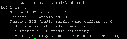We see 32 bbcredits. While for Brocade: there are only 8. Of course higher values are common, and often essential, for ISLs over distance, but these are fairly typical values. So, how do these numbers impact the performance of the 8Gb/s port in our model. We can use Little’s law to work out the queue length.

$L=\lambda.W$

Where L is the mean requests in the queue, $\lambda$ is the arrival rate, and W is the total time the request is in the queue. It can immediately be seen that $W = T - s$ , so:

$L=\lambda.(T-s)$

Now, the arrival rate must be:

$\lambda = \frac{\rho}{s}$

So, we now have:

$L=\frac{\rho.(T-s)}{s}$

and substituting back in the M/M/1 queuing formula from my previous post, we have:

$L=\frac{\rho}{s}.(\frac{s}{1-\rho}-s)$

Now, simplifying, we get a formula for the queue length wrt utilization and service time.

$L=\frac{\rho ^2}{(1-\rho).s}$

We can now graph the relationship between queue length and utilization for a service time of 2.5 microseconds:

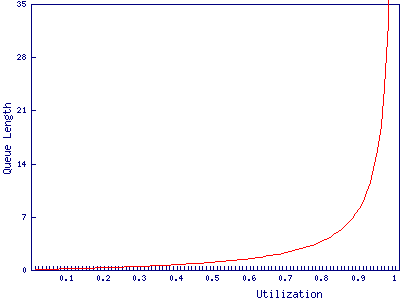
We find that the port with 8 buffers runs out of bbcredits just before 90% utilization, while the port with 32 buffers makes it to 97%. In and of itself a 7% difference in how heavily the port can be loaded may not be particularly important. It is after all only 573Mb/s, however, it may have wider implications for the fibre channel network due to the way buffer credits work.

A Simple Example

April 1, 2014 § 2 Comments

Taking an 8Gb/s fibre channel port, I’m going to use Queuing Theory, and some simplifying assumptions, to determine at what utilization latency becomes significant enough to worry about. Whether, and to what extent, these assumptions are justified is a discussion for another time. The aim is to make the analysis easy while still maintaining sufficient realism to be useful.

Let’s assume we are throwing data about and all our frames are carrying a full payload, giving a frame length of 2,112 bytes. With 8b/10b encoding, this ends up being 21,120 bits. 21,120 bits / 8Gb/s gives us an expected service time of 2.5 microseconds. To make this easier to deal with, we’ll assume the port has infinite buffers, that each frame arrives randomly and independently (a Poisson process) and that the service times are similarly distributed. None of these are entirely realistic assumptions, but they make it a lot easier to construct an analytical model.

With the above assumptions, we can use the formula for the responce time of an M/M/1 queue:

$T=(\frac{s}{1-\rho})$

Where $s$ is the time taken for the port to service the frame, and $\rho$ is utilization of the port.

If we plot this we find that the port appears to cope very well under high load:

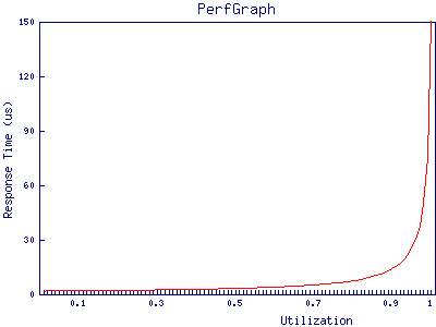
at 95% utilization, the port has only just hit 50 microseconds of response time. Given that the best case response time of a storage array is, in most cases, in the low hundreds of microseconds it’s clear that, in this example, queuing in the buffers on fibre channel ports can be discarded as a source of latency in all but the most extreme cases.

In future posts, I will explore ways in which this analysis can be extended and cases in which fibre channel network performance can impact storage performance.

ascknd

Analysing Experimental Results With R

Creating an Experimental Design in R

A Simple Example…With Finite Buffers

A Simple Example

Where Am I?