Perl PDQ: 8 core response time under load
May 15, 2014 § 1 Comment
The following Perl PDQ1; script was used to generate the response time data for the 8 core example in my https://ascknd.com/2014/05/02/nfs-vs-fibre-cpu-vmware/ post:
#/usr/bin/perl
use pdq;
$cores = $ARGV[0];
$servTime = $ARGV[1];
$max_rate = (1 / $servTime) * $cores;
print “response(secs)\t | util_%\n”;
for ($rate = 0; $rate < $max_rate ; $rate += $max_rate / 5) {
$arrivRate = $rate;
pdq::Init(“Open Network with M/M/N”);
pdq::SetComment(“Simulation of N CPU cores under transactional load.”);
pdq::CreateOpen(“work”, $arrivRate);
pdq::CreateMultiNode( $cores, “cores”, $pdq::CEN, $pdq::FCFS);
pdq::SetDemand(“cores”, “work”, $servTime);
pdq::SetWUnit(“IOS”);
pdq::SetTUnit(“Secs”);
pdq::Solve($pdq::CANON);
$response = substr(pdq::GetResponse($pdq::TRANS, “work”),0, 8);
$util = substr(pdq::GetUtilization(“cores”, “work”, $pdq::TRANS) * 100,0, 4);
printf “$response \t | % 4d\n”, $util;
}
perl ./mm8_response.pl 8 0.000127
response(secs) | util_%
0.000127 | 0
0.000127 | 20
0.000127 | 40
0.000132 | 60
0.000163 | 80
NFS vs Fibre Channel: Comparing CPU Utilization in VMWare
May 2, 2014 § 3 Comments
SUMMARY
Some years ago we were faced with the choice of which storage network protocol to use in our virtualized environment. Central to the discussion was a white paper, co-authored by Netapp and VMWare, comparing throughput and CPU utilization for NFS, FC and iSCSI. Broadly speaking the paper concluded that the differences in throughput were trivial, and for CPU utilization were under most circumstances small. At the time I wasn’t satisfied with the document, or indeed the conclusions that were able to drawn from it.
In this post, I will outline some work I performed recently using Queuing Theory1 and Design of Experiments2 to draw more specific conclusions from a broadly similar set of experiments to those undertaken by NetApp. I show that, if we restrict our analysis to storage efficiency in the hypervisor, in fact the choice of protocol is the dominant influence on CPU load, after IOPS (as can clearly be seen below in figure 4), and that under some circumstances, where latency of the order of 100μs is significant, or the total volume of IO is large, the choice of protocol can be an important determinant of performance, and potentially cost.
LIMITATIONS OF THE NETAPP PAPER
The white paper in question is NetApp document TR-36973. The equipment is more than a little out of date now, ESX 3.5, GigE, NetApp 2000 and 3000 series boxes and 2Gb FC-AL fibre. They ran 4K and 8K random and sequential workloads at various read/write ratios and at a range of thread counts. Tests were run to compare workloads over NFS, FC and iSCSI. For the purpose of this analysis, I ignore iSCSI and concentrate on NFS and FC.
In making use of this paper some issues become apparent:
1. All experimental results are scaled with respect to FC. This makes it hard to get a sense of what the result means in real terms, or to compare results between experiments.
2. The IOPS aren’t fixed between, or within, experiments. If response times increase, the IOPS, and hence the throughput, will tend to drop. This is observed in the results with NFS producing somewhat less throughput than FC under increased load.
If the IOPS are suppressed for NFS, then we might expect this also to keep the CPU utilization down, since there are fewer IOs for the CPU to process per unit of time. Despite this, the CPU is working harder for NFS.
3. By throttling based on the thread count, they are implicitly assuming closed queuing. This is not necessarily applicable to modeling transactional workloads.
4. Due to caching and interaction with the filesystem, it isn’t clear what IO is being processed by the VMWare IO subsystem. This will tend to minimize differences in the performance of the underlying infrastructure, since it is only being used a proportion of the time.
To progress with the analysis, fresh data is needed.
STEP 1: Test Configuration
I set up a small test configuration to run a similar set of experiments to those in the paper, though this time just comparing NFS and FC. There are some significant differences between the setup NetApp used and the one I built. Partly that is because technology has moved on since 2008, but most of the changes are because I have simplified the setup as far as possible.
The physical setup was as follows:

Figure 1
I ran a single minimally configured Debian guest running the 3.2.0-4-686-pae kernel inside an ESXi 5.5 (1331820) hypervisor. I configured a disk from an NFS datastore, and one from an FC datastore. The guest was assigned 8 vCPU and 1GB of memory.
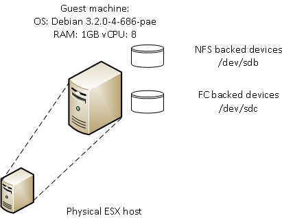
Figure 2
STEP 2: Workload Generation
In their test, NetApp used Iometer4 which throttles the workload based on thread count. Most freely available tools operate along the same lines as Iometer. To achieve the required level of control, I modified NetApp’s sio_ntap5 to hold a specified level of IOPS. A more detailed description of this work can be found here:
https://ascknd.com/2014/05/28/616/
I ran sio_ntap with the directio option set, bypassing cache and directed to a raw device. By doing this, different factors that directly influency the intensity of the workload can be compared and their effect quantified.
STEP 3: Experimental Design
NetApp consider a number of factors in their analysis – read%, random%, block size, protocol and thread count. I’m going to substitute IOPS for thread count. The response we are interested in is the CPU used by the ESX kernel (
In order to formulate a model of this system, it is necessary to make some assumptions:
1. An IO of any given type will take a fixed amount of CPU resources regardless of load.
1.1 We therefore expect to see all effects to involve a linear interaction with IOPS. This can readily be validated by plotting a graph showing the percentage of a CPU core used by the ESX kernel, as discussed above, for various workloads and IOPS:

Figure 3
It can readily be seen that NFS and FC diverge with plausibly linear behavior.
1.2 For any given read percent, or random percent, an IO is either read or write, random or sequential. We therefore expect their effect to be linear.
2. Since we are only interested in block sizes of 4 or 8, we will only consider linear effects of block size. No claims are made about applicability of the model to larger block sizes
3. Some background load will exist. This is assumed to be the load for zero IOPS. This will be deducted from all subsequent calculations for CPU load. Taking this into account, the previous graph can be amended so that the average CPU utilization at zero IOPS is zero:

Figure 4
All effects are therefore expected to be linear, to involve interactions with IOPS and go through the origin.
The following design will be used:
| read% | rand% | blk_sz | protocol | iops |
| 0 | 0 | 4 | fc | 1000 |
| 100 | 100 | 8 | nfs | 4000 |
Table 1
This gives a full factorial experimental design with 32 experiments. Repeating every experiment 20 times, 640 runs are needed.
| run | read% | rand% | blk_sz | protocol | iops |
| 1 | 0 | 100 | 4 | fc | 4000 |
| 2 | 0 | 0 | 8 | fc | 1000 |
| <snip> | |||||
| 639 | 0 | 0 | 4 | fc | 4000 |
| 640 | 0 | 0 | 8 | nfs | 1000 |
Table 2
A more detailed discussion on how to create the design in R is shown here:
We now need to run the modified sio_ntap tool with the above parameters 640 times and analyze the results.
STEP 4: Analysis of Results
R6 is used with the DoE7 package to analyze the results. This solves the experimental results as a system of simultaneous equation. A detailed explanation of this is presented here:
The analysis shows that we can approximate the CPU utilization, by the following equation for large IOPS:
Equation 1

Which implies that NFS is approximately 1.96 times as expensive in terms of CPU utilization as Fibre Channel (see linked article).
STEP 5: Real World Context
Whether this difference in the cost of NFS and FC IO is important, or not, depends on the extent to which it has a significant impact on macro level system characteristics that relate to the financial cost, and feasibility, of delivering on design requirements.
Solving equation 1 for a single IOP, we see that one NFS IO uses 
| response(secs) | util_% |
| 0.000081 | 0 |
| 0.000081 | 20 |
| 0.000081 | 40 |
| 0.000085 | 60 |
| 0.000104 | 80 |
Table 3
A typical midrange disk subsystem can turn around an IO in about 500μs. Some higher end subsystems can respond in 150μs, or less. So this is an effect that is of the same order of magnitude as other metrics that clearly can determine system performance.
These individual IOs add up of course. In this example, one CPU core can handle ~12K NFS IOPS, or 24K FC IOPS. This potentially has architectural and cost implications if a significant intensity of IO is being serviced. A 70K IOP requirement would require a 6 cores for NFS, but only 3 for FC, purely processing the IO in the hypervisor.
CONCLUSIONS
While NFS clearly induces more load on the ESX server than FC, to some degree these costs need to be seen in context. The reason the NetApp paper found a relatively small difference between the protocols is that there are many other factors contribute to the overall CPU load associated with doing IO. Often the cost within the hypervisor will be relatively insignificant:
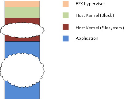
Figure 5
Whether the hypervisor is important depends on the interaction between the workload and each of these other elements. Analysing these interactions is a larger problem and not trivial to address in the general case.
1The Art of Computer Systems Performance Analysis, p.507 R. Jain, John Wiley & Sons Inc, 1991
2The Art of Computer Systems Performance Analysis, p.293 R. Jain, John Wiley & Sons Inc, 1991
3 Performance Report: Multiprotocol Performance Test of VMware® ESX 3.5 on NetApp Storage Systems, https://communities.vmware.com/servlet/JiveServlet/download/1085778-15260/NetApp_PerformanceTest_tr-3697.pdf, Jack McLeod, NetApp, June 2008
4 http://www.iometer.org/
5 https://communities.netapp.com/blogs/zurich/2011/01/24/sio–performance-load-testing-simplified
6 http://cran.r-project.org/
7 http://prof.beuth-hochschule.de/groemping/software/design-of-experiments/project-industrial-doe-in-r/
8 https://ascknd.com/2014/05/15/442/
Document Changes:
27/05/2014 – Updated experimental design with 20 replications instead of 5 and simplified the setup of the block devices. All equations and graphs modified to agree with new data. Some additional minor cosmetic changes and corrections.
A Simple Example…With Finite Buffers
April 4, 2014 § Leave a comment
As load increases on a service center, in the case of our earlier example – a fibre channel port, queues of requests form. These queues are held in the buffers of the port. In my first post, I assumed that the buffers were infinitely deep. That is clearly not the case for any real world implementation. Historically in fibre channel networks relatively few buffers were used when compared to Ethernet networks. Cisco has tended to have more buffers than Brocade. A typical value for Cisco is shown here: 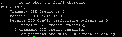 We see 32 bbcredits. While for Brocade:
  there are only 8. Of course higher values are common, and often essential, for ISLs over distance, but these are fairly typical values. So, how do these numbers impact the performance of the 8Gb/s port in our model. We can use Little’s law to work out the queue length.

Where L is the mean requests in the queue, 


Now, the arrival rate must be:

So, we now have:

and substituting back in the M/M/1 queuing formula from my previous post, we have:

Now, simplifying, we get a formula for the queue length wrt utilization and service time.

We can now graph the relationship between queue length and utilization for a service time of 2.5 microseconds:
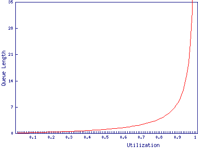
We find that the port with 8 buffers runs out of bbcredits just before 90% utilization, while the port with 32 buffers makes it to 97%. In and of itself a 7% difference in how heavily the port can be loaded may not be particularly important. It is after all only 573Mb/s, however, it may have wider implications for the fibre channel network due to the way buffer credits work.
A Simple Example
April 1, 2014 § 2 Comments
Taking an 8Gb/s fibre channel port, I’m going to use Queuing Theory, and some simplifying assumptions, to determine at what utilization latency becomes significant enough to worry about. Whether, and to what extent, these assumptions are justified is a discussion for another time. The aim is to make the analysis easy while still maintaining sufficient realism to be useful.
Let’s assume we are throwing data about and all our frames are carrying a full payload, giving a frame length of 2,112 bytes. With 8b/10b encoding, this ends up being 21,120 bits. 21,120 bits / 8Gb/s gives us an expected service time of 2.5 microseconds. To make this easier to deal with, we’ll assume the port has infinite buffers, that each frame arrives randomly and independently (a Poisson process) and that the service times are similarly distributed. None of these are entirely realistic assumptions, but they make it a lot easier to construct an analytical model.
With the above assumptions, we can use the formula for the responce time of an M/M/1 queue:

Where 

If we plot this we find that the port appears to cope very well under high load:
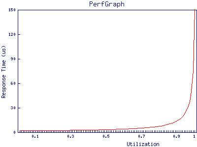
at 95% utilization, the port has only just hit 50 microseconds of response time. Given that the best case response time of a storage array is, in most cases, in the low hundreds of microseconds it’s clear that, in this example, queuing in the buffers on fibre channel ports can be discarded as a source of latency in all but the most extreme cases.
In future posts, I will explore ways in which this analysis can be extended and cases in which fibre channel network performance can impact storage performance.
