Helpdesk Queue Analyser PDQ::Perl
June 23, 2014 § 1 Comment
Below is a Perl script using the PDQ Perl module to analyser the performance of two helpdesk and predict their behaviour should their queues be merged.
A more complete discussion of the motivations for this and conclusions can be found here:
#/usr/bin/perl
use pdq;
use strict;
use warnings;
my $siteAStaff = $ARGV[0];
my $siteAServiceTime = $ARGV[1];
my $siteARate = $ARGV[2];
my $siteBStaff = $ARGV[3];
my $siteBServiceTime = $ARGV[4];
my $siteBRate = $ARGV[5];
#Handle site A
pdq::Init(“Open Network with M/M/N”);
pdq::SetComment(“Simulation of site A mean performance.”);
pdq::CreateOpen(“work”, $siteARate);
pdq::CreateMultiNode( $siteAStaff, “cores”, $pdq::CEN, $pdq::FCFS);
pdq::SetDemand(“cores”, “work”, $siteAServiceTime);
pdq::SetWUnit(“Calls”);
pdq::SetTUnit(“Mins”);
pdq::Solve($pdq::CANON);
my $responseA = substr(pdq::GetResponse($pdq::TRANS, “work”),0, 8);
my $utilA = substr(pdq::GetUtilization(“cores”, “work”, $pdq::TRANS) * 100,0, 4);
#Handle site B
pdq::Init(“Simulation of site B mean performance.”);
pdq::SetComment(“Simulation of 8 core CPU under transactional load.”);
pdq::CreateOpen(“work”, $siteBRate);
pdq::CreateMultiNode( $siteBStaff, “cores”, $pdq::CEN, $pdq::FCFS);
pdq::SetDemand(“cores”, “work”, $siteBServiceTime);
pdq::SetWUnit(“Calls”);
pdq::SetTUnit(“Mins”);
pdq::Solve($pdq::CANON);
my $responseB = substr(pdq::GetResponse($pdq::TRANS, “work”),0, 8);
my $utilB = substr(pdq::GetUtilization(“cores”, “work”, $pdq::TRANS) * 100,0, 4);
#Handle combined site
pdq::Init(“Open Network with M/M/N”);
pdq::SetComment(“Simulation of comined site mean performance.”);
pdq::CreateOpen(“work”, $siteARate + $siteBRate);
pdq::CreateMultiNode( $siteAStaff + $siteBStaff, “cores”, $pdq::CEN, $pdq::FCFS);
pdq::SetDemand(“cores”, “work”, ($siteAStaff * $siteAServiceTime + $siteBStaff * $siteBServiceTime) / ($siteAStaff + $siteBStaff) );
pdq::SetWUnit(“Calls”);
pdq::SetTUnit(“Mins”);
pdq::Solve($pdq::CANON);
my $responseAB = substr(pdq::GetResponse($pdq::TRANS, “work”),0, 8);
my $utilAB = substr(pdq::GetUtilization(“cores”, “work”, $pdq::TRANS) * 100,0, 4);
printf “Site \t| Response \t | utilization\n”;
printf “A \t| %f \t | % 4d\n”, $responseA, $utilA;
printf “B \t| %f \t | % 4d\n”, $responseB, $utilB;
printf “Combined\t| %f \t | % 4d\n”, $responseAB, $utilAB;
Syntax:
perl ./helpdesk_response.pl <siteA call helpdesk staff#> <siteA service time (mins)> <siteA calls per minute> <siteB call helpdesk staff#> <siteB service time (mins)> <siteB calls per minute>
NB: Service time is used here, not response time, so time spent in the queue doesn’t count. Response time is used in the outputted performance.
Example:
perl ./helpdesk_response.pl 4 30 0.08 6 30 .18
Site | Response | utilization
A | 35.382050 | 60
B | 67.006280 | 90
Combined | 34.990830 | 78
Perl PDQ: 8 core response time under load
May 15, 2014 § 1 Comment
The following Perl PDQ1; script was used to generate the response time data for the 8 core example in my https://ascknd.com/2014/05/02/nfs-vs-fibre-cpu-vmware/ post:
#/usr/bin/perl
use pdq;
$cores = $ARGV[0];
$servTime = $ARGV[1];
$max_rate = (1 / $servTime) * $cores;
print “response(secs)\t | util_%\n”;
for ($rate = 0; $rate < $max_rate ; $rate += $max_rate / 5) {
$arrivRate = $rate;
pdq::Init(“Open Network with M/M/N”);
pdq::SetComment(“Simulation of N CPU cores under transactional load.”);
pdq::CreateOpen(“work”, $arrivRate);
pdq::CreateMultiNode( $cores, “cores”, $pdq::CEN, $pdq::FCFS);
pdq::SetDemand(“cores”, “work”, $servTime);
pdq::SetWUnit(“IOS”);
pdq::SetTUnit(“Secs”);
pdq::Solve($pdq::CANON);
$response = substr(pdq::GetResponse($pdq::TRANS, “work”),0, 8);
$util = substr(pdq::GetUtilization(“cores”, “work”, $pdq::TRANS) * 100,0, 4);
printf “$response \t | % 4d\n”, $util;
}
perl ./mm8_response.pl 8 0.000127
response(secs) | util_%
0.000127 | 0
0.000127 | 20
0.000127 | 40
0.000132 | 60
0.000163 | 80
A Simple Example…With Finite Buffers
April 4, 2014 § Leave a comment
As load increases on a service center, in the case of our earlier example – a fibre channel port, queues of requests form. These queues are held in the buffers of the port. In my first post, I assumed that the buffers were infinitely deep. That is clearly not the case for any real world implementation. Historically in fibre channel networks relatively few buffers were used when compared to Ethernet networks. Cisco has tended to have more buffers than Brocade. A typical value for Cisco is shown here: 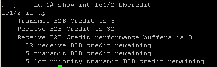 We see 32 bbcredits. While for Brocade:
  there are only 8. Of course higher values are common, and often essential, for ISLs over distance, but these are fairly typical values. So, how do these numbers impact the performance of the 8Gb/s port in our model. We can use Little’s law to work out the queue length.

Where L is the mean requests in the queue, 


Now, the arrival rate must be:

So, we now have:

and substituting back in the M/M/1 queuing formula from my previous post, we have:

Now, simplifying, we get a formula for the queue length wrt utilization and service time.

We can now graph the relationship between queue length and utilization for a service time of 2.5 microseconds:
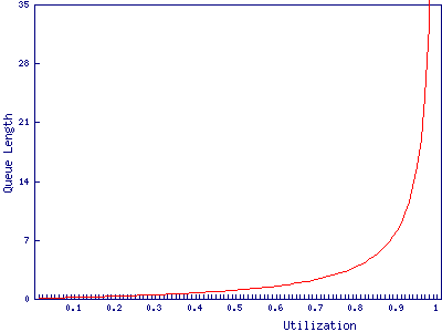
We find that the port with 8 buffers runs out of bbcredits just before 90% utilization, while the port with 32 buffers makes it to 97%. In and of itself a 7% difference in how heavily the port can be loaded may not be particularly important. It is after all only 573Mb/s, however, it may have wider implications for the fibre channel network due to the way buffer credits work.
A Simple Example
April 1, 2014 § 2 Comments
Taking an 8Gb/s fibre channel port, I’m going to use Queuing Theory, and some simplifying assumptions, to determine at what utilization latency becomes significant enough to worry about. Whether, and to what extent, these assumptions are justified is a discussion for another time. The aim is to make the analysis easy while still maintaining sufficient realism to be useful.
Let’s assume we are throwing data about and all our frames are carrying a full payload, giving a frame length of 2,112 bytes. With 8b/10b encoding, this ends up being 21,120 bits. 21,120 bits / 8Gb/s gives us an expected service time of 2.5 microseconds. To make this easier to deal with, we’ll assume the port has infinite buffers, that each frame arrives randomly and independently (a Poisson process) and that the service times are similarly distributed. None of these are entirely realistic assumptions, but they make it a lot easier to construct an analytical model.
With the above assumptions, we can use the formula for the responce time of an M/M/1 queue:

Where 

If we plot this we find that the port appears to cope very well under high load:
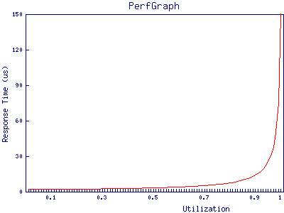
at 95% utilization, the port has only just hit 50 microseconds of response time. Given that the best case response time of a storage array is, in most cases, in the low hundreds of microseconds it’s clear that, in this example, queuing in the buffers on fibre channel ports can be discarded as a source of latency in all but the most extreme cases.
In future posts, I will explore ways in which this analysis can be extended and cases in which fibre channel network performance can impact storage performance.
